22 MySQL子查询优化策略
你好,我是俊达。
这一讲,我们来讨论子查询的一些优化策略。子查询是SQL很重要的一个能力,平时也不少见。
子查询的一个例子
早期MySQL(5.5以及更早的版本)对子查询的支持比较弱,使用子查询时容易遇到性能问题。
在13讲的思考题中,就有一个执行了几天都没有完成的SQL。
Command: Query
Time: 184551
State: Sending data
Info: select item_id, sum(sold) as sold
from stat_item_detail
where item_id in (
select item_id
from stat_item_detail
where gmt_create >= '2019-10-05 08:59:00')
group by item_id
上面这个SQL语句并不复杂,我们来构建一个测试表,准备一些数据,并做一些测试。使用下面这段SQL创建表,并写入100万行数据。
create table stat_item_detail(
id int not null auto_increment,
item_id int not null,
sold int not null,
gmt_create datetime not null,
padding varchar(4000),
primary key(id),
key idx_item_id(item_id),
key idx_gmt_create(gmt_create)
) engine=innodb;


create view digit
as select 0 as a union all select 1 union all select 2 union all select 3
union all select 4  union all select 5 union all select 6
union all select 7  union all select 8 union all select 9 ;

create view numbers_1m AS
select ((((a.a * 10 + b.a)*10 + c.a)*10 + d.a)*10+e.a)*10+f.a as n
from digit a, digit b, digit c, digit d, digit e, digit f;

insert into stat_item_detail(item_id, sold, gmt_create, padding)
select n + 1000000 - n % 2 as item_id,
n % 100 - n%100%2,
date_add('2024-06-01 00:00:00', interval n minute) as gmt_create,
rpad('x', 1000, 'abcdefg ') as padding
from numbers_1m;
当时用的还是MySQL 5.1和5.5的版本。我们先来看一下在5.5中这个SQL的执行计划。
mysql> explain select item_id, sum(sold) as sold
from stat_item_detail
where item_id in (
select item_id
from stat_item_detail
where Gmt_create >= '2026-04-26 10:30:00')
group by item_id;

+----+--------------------+------------------+----------------+----------------------------+-------------+---------+------+---------+-------------+
| id | select_type        | table            | type           | possible_keys              | key         | key_len | ref  | rows    | Extra       |
+----+--------------------+------------------+----------------+----------------------------+-------------+---------+------+---------+-------------+
|  1 | PRIMARY            | stat_item_detail | index          | NULL                       | idx_item_id | 4       | NULL | 1000029 | Using where |
|  2 | DEPENDENT SUBQUERY | stat_item_detail | index_subquery | idx_item_id,idx_gmt_create | idx_item_id | 4       | func |       1 | Using where |
+----+--------------------+------------------+----------------+----------------------------+-------------+---------+------+---------+-------------+
从上面的这个执行计划可以看到,这个SQL在执行时,先全量扫描索引idx_item_id,每得到一个item_id后,执行相关子查询(DEPENDENT SUBQUERY)select 1 from stat_item_detail where gmt_create >= ‘2026-04-26 10:30:00’ and item_id = primary.item_id。当主查询中表中的数据量很大的时候,子查询执行的次数也会很多,因此SQL的性能非常差。
在我的测试环境中,执行这个SQL需要45秒左右。
mysql> select item_id, sum(sold) as sold
from stat_item_detail
where item_id in (
select item_id
from stat_item_detail
where Gmt_create >= '2026-04-26 10:30:00')
group by item_id;
+---------+------+
| item_id | sold |
+---------+------+
| 1999990 |  180 |
| 1999992 |  184 |
| 1999994 |  188 |
| 1999996 |  192 |
| 1999998 |  196 |
+---------+------+
5 rows in set (44.64 sec)
那么将IN改成exists后,是否能提升性能呢?我们来试一下,可以看到执行时间和使用IN基本一样。
mysql> select item_id, sum(sold) as sold
from stat_item_detail t1
where exists (
select 1
from stat_item_detail
where gmt_create >= '2026-04-26 10:30:00'
and item_id = t1.item_id )
group by item_id;

+---------+------+
| item_id | sold |
+---------+------+
| 1999990 |  180 |
| 1999992 |  184 |
| 1999994 |  188 |
| 1999996 |  192 |
| 1999998 |  196 |
+---------+------+
5 rows in set (44.71 sec)
实际上,你会发现,不管是使用IN还是Exists,执行计划都是一样的。
mysql> explain select item_id, sum(sold) as sold
from stat_item_detail t1
where exists (
select 1
from stat_item_detail
where gmt_create >= '2026-04-26 10:30:00'
and item_id = t1.item_id )
group by item_id;
+----+--------------------+------------------+-------+----------------------------+-------------+---------+----------------+---------+-------------+
| id | select_type        | table            | type  | possible_keys              | key         | key_len | ref            | rows    | Extra       |
+----+--------------------+------------------+-------+----------------------------+-------------+---------+----------------+---------+-------------+
|  1 | PRIMARY            | t1               | index | NULL                       | idx_item_id | 4       | NULL           | 1000029 | Using where |
|  2 | DEPENDENT SUBQUERY | stat_item_detail | ref   | idx_item_id,idx_gmt_create | idx_item_id | 4       | rep.t1.item_id |       1 | Using where |
+----+--------------------+------------------+-------+----------------------------+-------------+---------+----------------+---------+-------------+
观察这个SQL最终返回的数据实际上并不多,因为子查询select item_id from stat_item_detail where gmt_create >= '2026-04-26 10:30:00’只需要返回最近写入的数据。
那么是不是可以先执行子查询呢?我们尝试改写一下SQL。改写后,查询的效率提高了很多,但是查询的结果有点问题了。
mysql> select t1.item_id, sum(t1.sold) as sold
from stat_item_detail t1, stat_item_detail t2
where t1.item_id = t2.item_id
and t2.gmt_create >= '2026-04-26 10:30:00'
group by t1.item_id;
+---------+------+
| item_id | sold |
+---------+------+
| 1999990 |  360 |
| 1999992 |  368 |
| 1999994 |  376 |
| 1999996 |  384 |
| 1999998 |  392 |
+---------+------+
5 rows in set (0.00 sec)
问题出在哪里呢?因为子查询中,item_id不是唯一的。改成普通的表连接后,数据有重复。因此我们需要对数据做一个去重。
select item_id, sum(sold) from (
select distinct t1.item_id, t1.sold as sold, t2.sold as sold2
from stat_item_detail t1, stat_item_detail t2
where t1.item_id = t2.item_id
and t2.gmt_create >= '2026-04-26 10:30:00'
) t group by item_id;
+---------+-----------+
| item_id | sum(sold) |
+---------+-----------+
| 1999990 |        90 |
| 1999992 |        92 |
| 1999994 |        94 |
| 1999996 |        96 |
| 1999998 |        98 |
+---------+-----------+
5 rows in set (0.00 sec)
但是,这样去重后,数据还是不对。因为主表中item_id是允许重复的,我们只需要对子查询中的item_id去重。将SQL改成下面这个样子,查询结果终于正确了,SQL的效率也还不错。
mysql> select t1.item_id, sum(t1.sold) as sold
from stat_item_detail t1, (
select distinct item_id
from stat_item_detail t2
where t2.gmt_create >= '2026-04-26 10:30:00') t22
where t1.item_id = t22.item_id
group by t1.item_id;
+---------+------+
| item_id | sold |
+---------+------+
| 1999990 |  180 |
| 1999992 |  184 |
| 1999994 |  188 |
| 1999996 |  192 |
| 1999998 |  196 |
+---------+------+
5 rows in set (0.00 sec)
实际上,我们还可以使用另外一种方法来去重,也就是按主表的主键字段来去重。
select item_id, sum(sold) from (
select distinct t1.id,  t1.item_id, t1.sold as sold
from stat_item_detail t1, stat_item_detail t2
where t1.item_id = t2.item_id
and t2.gmt_create >= '2026-04-26 10:30:00'
) t group by item_id;

+---------+-----------+
| item_id | sum(sold) |
+---------+-----------+
| 1999990 |       180 |
| 1999992 |       184 |
| 1999994 |       188 |
| 1999996 |       192 |
| 1999998 |       196 |
+---------+-----------+
5 rows in set (0.00 sec)
MySQL的半连接(SEMIJOIN)优化
MySQL 5.6开始引入了半连接转换,对于前面例子中的SQL,优化器会自动进行查询转换,不需要再手动改写SQL了。在MySQL 5.6和5.7中,还不会对exists做半连接优化。从MySQL 8.0.16开始,优化器对exists子查询也会进行半连接转换。
在8.0的环境中执行这个SQL,MySQL自动把查询转换成了半连接。
mysql> explain select item_id, sum(sold) as sold
from stat_item_detail
where item_id in (
select item_id
from stat_item_detail
where Gmt_create >= '2026-04-26 10:30:00')
group by item_id;

+----+--------------+------------------+-------+----------------------------+----------------+---------+---------------------+------+----------+-----------------------+
| id | select_type  | table            | type  | possible_keys              | key            | key_len | ref                 | rows | filtered | Extra                 |
+----+--------------+------------------+-------+----------------------------+----------------+---------+---------------------+------+----------+-----------------------+
|  1 | SIMPLE       | <subquery2>      | ALL   | NULL                       | NULL           | NULL    | NULL                | NULL |   100.00 | Using temporary       |
|  1 | SIMPLE       | stat_item_detail | ref   | idx_item_id                | idx_item_id    | 4       | <subquery2>.item_id |    1 |   100.00 | NULL                  |
|  2 | MATERIALIZED | stat_item_detail | range | idx_item_id,idx_gmt_create | idx_gmt_create | 5       | NULL                |   10 |   100.00 | Using index condition |
+----+--------------+------------------+-------+----------------------------+----------------+---------+---------------------+------+----------+-----------------------+
上面的这个执行计划,实际上和我们的第一种手动改写的方式类似。
mysql> select t1.item_id, sum(t1.sold) as sold
from stat_item_detail t1, (
select distinct item_id
from stat_item_detail t2
where t2.gmt_create >= '2026-04-26 10:30:00') t22
where t1.item_id = t22.item_id
group by t1.item_id;

+----+-------------+------------+-------+----------------------------+----------------+---------+-------------+------+----------+----------------------------------------+
| id | select_type | table      | type  | possible_keys              | key            | key_len | ref         | rows | filtered | Extra                                  |
+----+-------------+------------+-------+----------------------------+----------------+---------+-------------+------+----------+----------------------------------------+
|  1 | PRIMARY     | <derived2> | ALL   | NULL                       | NULL           | NULL    | NULL        |   10 |   100.00 | Using temporary                        |
|  1 | PRIMARY     | t1         | ref   | idx_item_id                | idx_item_id    | 4       | t22.item_id |    1 |   100.00 | NULL                                   |
|  2 | DERIVED     | t2         | range | idx_item_id,idx_gmt_create | idx_gmt_create | 5       | NULL        |   10 |   100.00 | Using index condition; Using temporary |
+----+-------------+------------+-------+----------------------------+----------------+---------+-------------+------+----------+----------------------------------------+
当然,能进行半连接转换的SQL,需要满足一些基本的条件。
- 子查询没有使用UNION。
- 子查询没有使用Having。
- 子查询没有使用聚合函数(如avg、sum等)。
- 子查询中不允许使用limit。
- 主查询和子查询没有使用STRAIGHT_JOIN。
- 主查询中表的数量和子查询中表的数量相加不超过MySQL允许的最大表连接数量。MySQL最多允许61表的连接。
子查询中可以使用distinct、order by、group by这些关键词,实际上子查询中的这些关键词会被优化器忽略掉(前提是没有同时使用了聚合函数)。
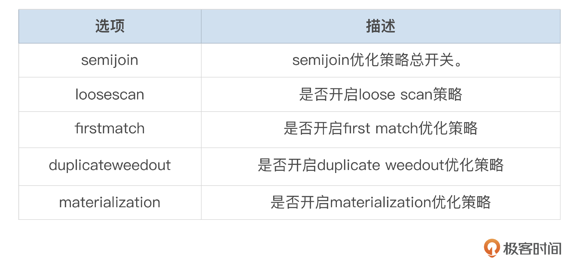
如果子查询满足了上面这些条件,优化器会自动查询转换,将子查询转换为半连接。优化器会根据语句的具体情况,选择合适策略来执行半连接。这些策略分别是pullout、duplicate weedout、first match、loose scan、materialization。
- Pullout:直接将子查询提到外层,改写成表连接。
- Duplicate weedout:如果子查询中的数据可能存在重复,MySQL会对结果数据进行去重。
- First Match:执行表连接时,对于驱动表中的每一行记录,只需要匹配子查询的第一条记录就返回。
- Loose Scan:利用子查询中索引的有序性,获取关联条件的唯一值。
- Materialization:将子查询的结果存储在临时表,临时表再和父表进行关联。
参数optimizer_switch中有一些选项用来控制是否开启某个半连接策略,我整理成了下面这个表格。
优化器会计算这些半连接策略的成本,从中选择成本最低的执行计划。
接下来我用一些具体的例子来说明这些执行策略的使用场景。
先根据下面的SQL,创建几个测试表,准备一些测试数据。
CREATE TABLE t_parent (
id int not null auto_increment,
a int,
b int ,
c int ,
padding varchar(2000),
primary key(id),
KEY idx_a (a)
) ENGINE=InnoDB;

CREATE TABLE t_subq (
id int not null auto_increment,
a int ,
b int ,
c int ,
d int ,
padding varchar(2000),
primary key(id),
UNIQUE KEY uk_cb (c,b),
KEY idx_abc (a,b,c)
) ENGINE=InnoDB;

insert into t_parent(a,b,c) values
(1,1,1),(2,2,2),(3,3,3),(4,4,4),(5,5,5),(null,0,0),(2,2,2);

insert into t_subq (a,b,c,d) values
(1,1,1,1),(2,2,2,2),(3,3,3,3),(2,4,4,2);
Pullout
如果子查询中,表上的唯一索引或主键能保证数据的唯一性,就可以直接将子查询转换为表连接,不用做其他额外的处理,这种转换就叫做Pullout,下面的查询演示了这种情况。
mysql> explain select * from t_parent where a in (
select b from t_subq where c = 1);

+----+-------------+----------+------+---------------+-------+---------+--------------+------+----------+--------------------------+
| id | select_type | table    | type | possible_keys | key   | key_len | ref          | rows | filtered | Extra                    |
+----+-------------+----------+------+---------------+-------+---------+--------------+------+----------+--------------------------+
|  1 | SIMPLE      | t_subq   | ref  | uk_cb         | uk_cb | 5       | const        |    1 |   100.00 | Using where; Using index |
|  1 | SIMPLE      | t_parent | ref  | idx_a         | idx_a | 5       | rep.t_subq.b |    1 |   100.00 | NULL                     |
+----+-------------+----------+------+---------------+-------+---------+--------------+------+----------+--------------------------+
由于子查询内的ty表上有唯一索引uk_cb(c,b),在c=1的情况下,b是唯一的,所以直接将子查询转换成了表连接。
执行show warnings后,可以看到SQL已经被改写成了普通的表连接。
mysql> show warnings\G
*************************** 1. row ***************************
Level: Note
Code: 1003
Message: /* select#1 */ select `rep`.`t_parent`.`id` AS `id`,`rep`.`t_parent`.`a` AS `a`,`rep`.`t_parent`.`b` AS `b`,`rep`.`t_parent`.`c` AS `c`,`rep`.`t_parent`.`padding` AS `padding` from `rep`.`t_subq` join `rep`.`t_parent` where ((`rep`.`t_parent`.`a` = `rep`.`t_subq`.`b`) and (`rep`.`t_subq`.`c` = 1))
Duplicate Weedout
如果子查询中的数据有可能出现重复值,那么将子查询转换为表连接时,需要对子查询的数据进行去重,这种情况为Duplicate Weedout,下面是一个例子:
mysql>  explain  select * from t_parent where a in (
select d from t_subq where a in (1,3));
+----+-------------+----------+-------+---------------+---------+---------+--------------+------+----------+-----------------------------------------------------+
| id | select_type | table    | type  | possible_keys | key     | key_len | ref          | rows | filtered | Extra                                               |
+----+-------------+----------+-------+---------------+---------+---------+--------------+------+----------+-----------------------------------------------------+
|  1 | SIMPLE      | t_subq   | range | idx_abc       | idx_abc | 5       | NULL         |    2 |   100.00 | Using index condition; Using where; Start temporary |
|  1 | SIMPLE      | t_parent | ref   | idx_a         | idx_a   | 5       | rep.t_subq.d |    1 |   100.00 | End temporary                                       |
+----+-------------+----------+-------+---------------+---------+---------+--------------+------+----------+-----------------------------------------------------+
注意到执行计划中,select_type列显示SIMPLE,说明子查询已经被转换成表连接了。Extra列中的Start temporary和End temporary说明使用了临时表来对数据进行去重。这里会使用t_parent表的主键字段来去重。
执行show warnings可以看到转换后的查询使用了semi join。
mysql> show warnings\G
*************************** 1. row ***************************
Level: Note
Code: 1003
Message: /* select#1 */ select `rep`.`t_parent`.`id` AS `id`,`rep`.`t_parent`.`a` AS `a`,`rep`.`t_parent`.`b` AS `b`,`rep`.`t_parent`.`c` AS `c`,`rep`.`t_parent`.`padding` AS `padding` from `rep`.`t_parent` semi join (`rep`.`t_subq`) where ((`rep`.`t_parent`.`a` = `rep`.`t_subq`.`d`) and (`rep`.`t_subq`.`a` in (1,3)))
1 row in set (0.00 sec)
First match
子查询转换为半连接后,如果优化器选择以原先的主查询作为驱动表,还可以使用First match策略。First match的意思是,对于驱动表的每一行数据,关联子查询中的表时,只关联到1行数据就返回,这样就不需要对子查询中的数据进行去重处理了。下面是使用First match的一个例子:
mysql> explain select * from t_parent where c in (select c from t_subq);
+----+-------------+----------+------+---------------+-------+---------+----------------+------+----------+-----------------------------------+
| id | select_type | table    | type | possible_keys | key   | key_len | ref            | rows | filtered | Extra                             |
+----+-------------+----------+------+---------------+-------+---------+----------------+------+----------+-----------------------------------+
|  1 | SIMPLE      | t_parent | ALL  | NULL          | NULL  | NULL    | NULL           |    7 |   100.00 | Using where                       |
|  1 | SIMPLE      | t_subq   | ref  | uk_cb         | uk_cb | 5       | rep.t_parent.c |    1 |   100.00 | Using index; FirstMatch(t_parent) |
+----+-------------+----------+------+---------------+-------+---------+----------------+------+----------+-----------------------------------+
注意到上面的执行计划中,Extra列显示的FirstMatch(t_parent)。First Match和Duplicate Weedout的一个主要的区别是表连接的顺序不一样。如果以子查询中的表作为驱动表,就无法使用First Match策略了。
LooseScan
LooseScan策略会利用子查询中表上的索引来获取到一组唯一的值,再跟主查询中的表进行连接。下面是使用LooseScan的一个例子:
mysql> explain  select * from t_parent where a in (select a from t_subq);
+----+-------------+----------+-------+---------------+---------+---------+--------------+------+----------+-------------------------------------+
| id | select_type | table    | type  | possible_keys | key     | key_len | ref          | rows | filtered | Extra                               |
+----+-------------+----------+-------+---------------+---------+---------+--------------+------+----------+-------------------------------------+
|  1 | SIMPLE      | t_subq   | index | idx_abc       | idx_abc | 15      | NULL         |    4 |   100.00 | Using where; Using index; LooseScan |
|  1 | SIMPLE      | t_parent | ref   | idx_a         | idx_a   | 5       | rep.t_subq.a |    1 |   100.00 | NULL                                |
+----+-------------+----------+-------+---------------+---------+---------+--------------+------+----------+-------------------------------------+
注意到上面的执行计划Extra中显示的LooseScan,使用了t_subq表上的索引idx_abc获取到a的一系列唯一值,这种方式和索引跳跃扫描(index skip scan)有一些相似之处。使用LooseScan策略时,以子查询中的表作为驱动表。
Materialize with deduplication
在Materialize with deduplication这种策略下,子查询被物化(Materialize)成一个临时表,生成临时表的时候会同时对数据进行去重。去重后的临时表再和原先主查询中的表进行连接。下面就是使用这种策略的一个例子:
mysql> explain  select * from t_parent where a in (select d from t_subq where a in (2));
+----+--------------+-------------+------+---------------+---------+---------+---------------+------+----------+-------------+
| id | select_type  | table       | type | possible_keys | key     | key_len | ref           | rows | filtered | Extra       |
+----+--------------+-------------+------+---------------+---------+---------+---------------+------+----------+-------------+
|  1 | SIMPLE       | <subquery2> | ALL  | NULL          | NULL    | NULL    | NULL          | NULL |   100.00 | Using where |
|  1 | SIMPLE       | t_parent    | ref  | idx_a         | idx_a   | 5       | <subquery2>.d |    1 |   100.00 | NULL        |
|  2 | MATERIALIZED | t_subq      | ref  | idx_abc       | idx_abc | 5       | const         |    2 |   100.00 | NULL        |
+----+--------------+-------------+------+---------------+---------+---------+---------------+------+----------+-------------+
注意到上面执行计划中ID为2的查询单元,select_type为MATERIALIZED,这是基于子查询中的表t_subq产生的临时表。
半连接策略的执行成本
使用Pullout策略时,子查询中需要有主键或唯一索引来保证数据的唯一性。使用LooseScan策略时,也需要子查询中有索引。其他几种策略,对子查询中的索引没有要求。
那么在执行一个具体的子查询时,优化器是怎么来选择半连接策略的呢?实际上在这里,优化器主要也是基于成本来选择执行策略。每一种半连接转换策略都有相应的成本计算方式。我们可以使用优化器跟踪,来看一下子查询策略的选择过程。
mysql> set optimizer_trace='enabled=on';
Query OK, 0 rows affected (0.00 sec)

mysql> explain select item_id, sum(sold) as sold
from stat_item_detail
where item_id in (
select item_id
from stat_item_detail
where gmt_create >= '2026-04-26 10:30:00')
group by item_id;

+----+--------------+------------------+-------+----------------------------+----------------+---------+---------------------+------+----------+-----------------------+
| id | select_type  | table            | type  | possible_keys              | key            | key_len | ref                 | rows | filtered | Extra                 |
+----+--------------+------------------+-------+----------------------------+----------------+---------+---------------------+------+----------+-----------------------+
|  1 | SIMPLE       | <subquery2>      | ALL   | NULL                       | NULL           | NULL    | NULL                | NULL |   100.00 | Using temporary       |
|  1 | SIMPLE       | stat_item_detail | ref   | idx_item_id                | idx_item_id    | 4       | <subquery2>.item_id |    1 |   100.00 | NULL                  |
|  2 | MATERIALIZED | stat_item_detail | range | idx_item_id,idx_gmt_create | idx_gmt_create | 5       | NULL                |   10 |   100.00 | Using index condition |
+----+--------------+------------------+-------+----------------------------+----------------+---------+---------------------+------+----------+-----------------------+

mysql> select * from information_schema.optimizer_trace\G
- LooseScan
子查询中没有合适的索引可以用来执行LooseScan策略。
- MaterializeScan的成本
MaterializeScan的成本主要是创建临时表的成本,以及往临时表写入数据的成本。需要写入临时表的记录通过访问索引idx_gmt_create得到,需要写入10行记录。
"execution_plan_for_potential_materialization": {
"steps": [
{
"considered_execution_plans": [
{
"plan_prefix": [
],
"table": "`stat_item_detail`",
"best_access_path": {
"considered_access_paths": [
{
"access_type": "ref",
"index": "idx_item_id",
"usable": false,
"chosen": false
},
{
"rows_to_scan": 10,
"filtering_effect": [
],
"final_filtering_effect": 1,
"access_type": "range",
"range_details": {
"used_index": "idx_gmt_create"
},
"resulting_rows": 10,
"cost": 12.5992,
"chosen": true
}
]
},
"condition_filtering_pct": 100,
"rows_for_plan": 10,
"cost_for_plan": 12.5992,
"sort_cost": 10,
"new_cost_for_plan": 22.5992,
"chosen": true
}
]
}
]
}
再关联主表,得到执行计划的总成本为35.6627。
{
"strategy": "MaterializeScan",
"recalculate_access_paths_and_cost": {
"tables": [
{
"table": "`stat_item_detail`",
"best_access_path": {
"considered_access_paths": [
{
"access_type": "ref",
"index": "idx_item_id",
"rows": 1.88804,
"cost": 20.0634,
"chosen": true
},
{
"access_type": "scan",
"cost": 159249,
"rows": 903690,
"chosen": false,
"cause": "cost"
}
]
}
}
]
},
"cost": 35.6627,
"rows": 1.88804,
"duplicate_tables_left": true,
"chosen": true
}
- DuplicatesWeedout的成本
DuplicatesWeedout的成本,由正常的表连接成本和去重成本组成,去重的成本为创建临时表的成本加上往临时表中写入数据的成本。从优化器跟踪可以看到,使用DuplicatesWeedout策略时,查询的总成本为37.4387,超过了Materialize的成本,因此没有选择这个策略。
{
"strategy": "DuplicatesWeedout",
"cost": 37.4387,
"rows": 18.8804,
"duplicate_tables_left": false,
"chosen": false
}
- 主查询作为驱动表的成本
使用FirstMatch时,以原先的主查询作为驱动表,访问主表时,需要全表扫描,成本超过了之前Materialize的成本,因此也没有选择这个执行计划。
{
"plan_prefix": [
],
"table": "`stat_item_detail`",
"best_access_path": {
"considered_access_paths": [
{
"access_type": "ref",
"index": "idx_item_id",
"usable": false,
"chosen": false
},
{
"rows_to_scan": 903690,
"filtering_effect": [
],
"final_filtering_effect": 1,
"access_type": "scan",
"resulting_rows": 903690,
"cost": 159249,
"chosen": true,
"use_tmp_table": true
}
]
},
"condition_filtering_pct": 100,
"rows_for_plan": 903690,
"cost_for_plan": 159249,
"semijoin_strategy_choice": [
],
"pruned_by_cost": true
}
反连接(ANTI Join)简介
按官方文档的说法,MySQL 8.0.17开始,对于满足半连接转换条件的not in、not exists查询,MySQL还会使用反查询(ANTI Join)转换。
但是在我的测试中,not in的执行计划中仍旧是相关子查询(DEPENDENT SUBQUERY)。
mysql> explain select * from t_parent
where b not in (
select b from t_subq where b is not null
);
+----+--------------------+----------+-------+---------------+-------+---------+------+------+----------+--------------------------+
| id | select_type        | table    | type  | possible_keys | key   | key_len | ref  | rows | filtered | Extra                    |
+----+--------------------+----------+-------+---------------+-------+---------+------+------+----------+--------------------------+
|  1 | PRIMARY            | t_parent | ALL   | NULL          | NULL  | NULL    | NULL |    7 |   100.00 | Using where              |
|  2 | DEPENDENT SUBQUERY | t_subq   | index | NULL          | uk_cb | 10      | NULL |    3 |    66.67 | Using where; Using index |
+----+--------------------+----------+-------+---------------+-------+---------+------+------+----------+--------------------------+
给主查询的not in字段加上not null条件后,查询才转换成了反连接。
mysql> explain select * from t_parent
where not exists (
select 1 from t_subq where a=t_parent.a)
and a is not null;
+----+-------------+----------+-------+---------------+---------+---------+----------------+------+----------+--------------------------------------+
| id | select_type | table    | type  | possible_keys | key     | key_len | ref            | rows | filtered | Extra                                |
+----+-------------+----------+-------+---------------+---------+---------+----------------+------+----------+--------------------------------------+
|  1 | SIMPLE      | t_parent | range | idx_a         | idx_a   | 5       | NULL           |    6 |   100.00 | Using index condition                |
|  1 | SIMPLE      | t_subq   | ref   | idx_abc       | idx_abc | 5       | rep.t_parent.a |    1 |   100.00 | Using where; Not exists; Using index |
+----+-------------+----------+-------+---------------+---------+---------+----------------+------+----------+--------------------------------------+

mysql> show warnings\G
*************************** 2. row ***************************
Level: Note
Code: 1003
Message: /* select#1 */ select `rep`.`t_parent`.`id` AS `id`,
`rep`.`t_parent`.`a` AS `a`,`rep`.`t_parent`.`b` AS `b`,
`rep`.`t_parent`.`c` AS `c`,`rep`.`t_parent`.`padding` AS `padding`
from `rep`.`t_parent` anti join (`rep`.`t_subq`)
on((`rep`.`t_subq`.`a` = `rep`.`t_parent`.`a`))
where (`rep`.`t_parent`.`a` is not null)
关于反连接,有一点需要注意,就是not in和not exists并不完全等价。如果子查询中存在NULL值,那么not in不会返回任何数据。
我们来执行一个简单的测试,子表t_subq写入一条null的数据。
mysql> insert into t_subq values(5,null, 0,0,0,null);
Query OK, 1 row affected (0.25 sec)

mysql> select * from t_parent;
+----+------+------+------+---------+
| id | a    | b    | c    | padding |
+----+------+------+------+---------+
|  1 |    1 |    1 |    1 | NULL    |
|  2 |    2 |    2 |    2 | NULL    |
|  3 |    3 |    3 |    3 | NULL    |
|  4 |    4 |    4 |    4 | NULL    |
|  5 |    5 |    5 |    5 | NULL    |
|  6 | NULL |    0 |    0 | NULL    |
|  7 |    2 |    2 |    2 | NULL    |
+----+------+------+------+---------+
7 rows in set (0.00 sec)

mysql> select * from t_subq;
+----+------+------+------+------+---------+
| id | a    | b    | c    | d    | padding |
+----+------+------+------+------+---------+
|  1 |    1 |    1 |    1 |    1 | NULL    |
|  2 |    2 |    2 |    2 |    2 | NULL    |
|  3 |    3 |    3 |    3 |    3 | NULL    |
|  4 |    2 |    4 |    4 |    2 | NULL    |
|  5 | NULL |    0 |    0 |    0 | NULL    |
+----+------+------+------+------+---------+
使用not in时,查询没有返回任何数据。这一点是使用not in时需要注意的。这是由not in和null的语意决定的,不光是MySQL,在其他数据库中也是一样的。
使用not exists时,可以查询到数据。
mysql> select * from t_parent where not exists (
select 1 from t_subq where a=t_parent.a);
+----+------+------+------+---------+
| id | a    | b    | c    | padding |
+----+------+------+------+---------+
|  4 |    4 |    4 |    4 | NULL    |
|  5 |    5 |    5 |    5 | NULL    |
|  6 | NULL |    0 |    0 | NULL    |
+----+------+------+------+---------+
子查询中需要增加not null条件,not in才能查询到数据。但是和not exists返回的数据还是有一点不同,就是not exists查询返回了主表中关联字段为null的数据。
mysql> select * from t_parent where a not in (
select a from t_subq where a is not null);
+----+------+------+------+---------+
| id | a    | b    | c    | padding |
+----+------+------+------+---------+
|  4 |    4 |    4 |    4 | NULL    |
|  5 |    5 |    5 |    5 | NULL    |
+----+------+------+------+---------+
无法使用半连接优化的子查询
MySQL中,子查询可以出现在语句的不同部分。子查询可以出现在Where条件中,一般以exists、not exists、in、not in的形式出现,这种情况前面我们已经做了一些讨论了。子查询还可以出现在SELECT的字段列表中,或者出现在FROM子句中,FROM子句中的子查询一般也称为派生表。
有些情况下,MySQL无法使用半连接转换来自动优化子查询,比如当子查询出现在select的列表中,或者子查询中使用了聚合函数。这些情况下,你可能需要手动改写SQL,来优化性能。
我们来举几个例子。先创建一个测试表,写入一些数据。
create table emp_salary(
id int not null auto_increment,
emp_id int not null,
dept_id int not null,
salary int not null,
padding varchar(2000),
primary key(id),
key idx_emp_id(emp_id),
key idx_dept_id(dept_id)
) engine=innodb;

insert into emp_salary(emp_id, dept_id, salary, padding)
select 100000 + n, n % 10, 10000 + (n * n) % 10000, rpad('A', 1000, 'ABCD')
from numbers;
下面这个SQL,子查询中使用了聚合函数,优化器无法使用半连接转换。
mysql> explain select * from emp_salary t1
where salary > (select avg(salary)
from emp_salary
where dept_id = t1.dept_id)

+----+--------------------+------------+------+---------------+-------------+---------+-----------------+------+----------+-------------+
| id | select_type        | table      | type | possible_keys | key         | key_len | ref             | rows | filtered | Extra       |
+----+--------------------+------------+------+---------------+-------------+---------+-----------------+------+----------+-------------+
|  1 | PRIMARY            | t1         | ALL  | NULL          | NULL        | NULL    | NULL            | 9295 |   100.00 | Using where |
|  2 | DEPENDENT SUBQUERY | emp_salary | ref  | idx_dept_id   | idx_dept_id | 4       | test.t1.dept_id |  929 |   100.00 | NULL        |
+----+--------------------+------------+------+---------------+-------------+---------+-----------------+------+----------+-------------+
在我的测试环境中,执行这个SQL需要大约执行9秒,原因主要是子查询执行的次数比较多。
类似的,下面这个SQL也需要执行9秒。
mysql> explain select * from (
select t1.emp_id, t1.dept_id, t1.salary,
(select avg(salary)
from emp_salary where dept_id = t1.dept_id
) as dept_avg_salary
from emp_salary t1 ) t
where salary > dept_avg_salary;

+----+--------------------+------------+------+---------------+-------------+---------+-----------------+------+----------+-------------+
| id | select_type        | table      | type | possible_keys | key         | key_len | ref             | rows | filtered | Extra       |
+----+--------------------+------------+------+---------------+-------------+---------+-----------------+------+----------+-------------+
|  1 | PRIMARY            | <derived2> | ALL  | NULL          | NULL        | NULL    | NULL            | 9295 |    33.33 | Using where |
|  2 | DERIVED            | t1         | ALL  | NULL          | NULL        | NULL    | NULL            | 9295 |   100.00 | NULL        |
|  3 | DEPENDENT SUBQUERY | emp_salary | ref  | idx_dept_id   | idx_dept_id | 4       | test.t1.dept_id |  929 |   100.00 | NULL        |
+----+--------------------+------------+------+---------------+-------------+---------+-----------------+------+----------+-------------+
对于这样的SQL,我们可以尝试改写,将相关子查询改成不相关子查询,这样可以减少子查询的执行次数。
mysql> select t1.*
from emp_salary t1,  (
select dept_id, avg(salary) as avg_salary
from emp_salary
group by dept_id ) t2
where t1.dept_id = t2.dept_id
and t1.salary > t2.avg_salary;

+----+-------------+------------+-------+---------------+-------------+---------+-----------------+------+----------+--------------------------+
| id | select_type | table      | type  | possible_keys | key         | key_len | ref             | rows | filtered | Extra                    |
+----+-------------+------------+-------+---------------+-------------+---------+-----------------+------+----------+--------------------------+
|  1 | PRIMARY     | t1         | ALL   | idx_dept_id   | NULL        | NULL    | NULL            | 9295 |   100.00 | NULL                     |
|  1 | PRIMARY     | <derived2> | ref   | <auto_key0>   | <auto_key0> | 4       | test.t1.dept_id |   92 |    33.33 | Using where; Using index |
|  2 | DERIVED     | emp_salary | index | idx_dept_id   | idx_dept_id | 4       | NULL            | 9295 |   100.00 | NULL                     |
+----+-------------+------------+-------+---------------+-------------+---------+-----------------+------+----------+--------------------------+
按上面这个方式改写后,SQL的执行效率提升了很多倍。你也可以到自己的环境中验证一下。还可以对比一下这几个SQL在慢日志中的Rows_examined指标。
总结
MySQL 8.0增强了子查询的优化能力,对很多简单的子查询,优化器可以自动处理。如果你在子查询中使用了聚合函数,或者在select字段中使用了子查询,可能需要进行手动的优化。使用not in时,要注意子查询中不要出现null的数据,这会导致查询不到任何数据。
思考题
这一讲中,我提供了两种手动改写子查询的思路。
思路1:
mysql> select t1.item_id, sum(t1.sold) as sold
from stat_item_detail t1, (
select distinct item_id
from stat_item_detail t2
where t2.gmt_create >= '2026-04-26 10:30:00') t22
where t1.item_id = t22.item_id
group by t1.item_id;
思路2:
select item_id, sum(sold) from (
select distinct t1.id,  t1.item_id, t1.sold as sold
from stat_item_detail t1, stat_item_detail t2
where t1.item_id = t2.item_id
and t2.gmt_create >= '2026-04-26 10:30:00'
) t group by item_id;
请问这两种改写方式,分别对应了MySQL半连接转换中的哪一个策略?
期待你的思考,欢迎你在留言区中与我交流。如果今天的课程让你有所收获,也欢迎转发给有需要的朋友。我们下节课再见!
- 叶明 👍(1) 💬(1)
思路1 +----+-------------+------------+------------+-------+----------------------------------------+ | id | select_type | table | partitions | type | Extra | +----+-------------+------------+------------+-------+----------------------------------------+ | 1 | PRIMARY | <derived2> | NULL | ALL | Using temporary | | 1 | PRIMARY | t1 | NULL | ref | NULL | | 2 | DERIVED | t2 | NULL | range | Using index condition; Using temporary | +----+-------------+------------+------------+-------+----------------------------------------+ 第一种改写方式对应半连接转换中的 Materialize with deduplication 策略, 从 distinct item_id 的语义和执行计划中 Extra 列中的 Using temporary,再通过执行计划的执行顺序可知,先生成一个内存临时表,将 item_id 列设置为唯一键, 然后范围扫描索引 idx_gmt_create ,将满足查询条件的 item_id 插入到表中。插入完成后,用该临时表与表 stat_item_detail 进行 join 操作。 这个过程与 materialize with deduplication 策略的过程一样——先将子查询物化成一个临时表,然后对临时表中的记录进行去重操作,最后将去重后的临时表与原主查询中的表进行关联查询。 思路2 +----+-------------+------------+------------+-------+----------------------------------------+ | id | select_type | table | partitions | type | Extra | +----+-------------+------------+------------+-------+----------------------------------------+ | 1 | PRIMARY | <derived2> | NULL | ALL | Using temporary | | 2 | DERIVED | t2 | NULL | range | Using index condition; Using temporary | | 2 | DERIVED | t1 | NULL | ref | NULL | +----+-------------+------------+------------+-------+----------------------------------------+ 第二种改写方式对应半连接转换中的 Duplicate Weedout 策略,使用到了内存临时表,并用主键来去重。
2024-10-12 - 陈星宇(2.11) 👍(0) 💬(1)
这些策略分别是 pullout、duplicate weedout、first match、loose scan、materialization。 这些是8.0才有吗?在5.7里很少看到。
2024-10-11 - 陈星宇(2.11) 👍(0) 💬(1)
mysql> explain select item_id, sum(sold) as sold from stat_item_detail where item_id in ( select item_id from stat_item_detail where Gmt_create >= '2026-04-26 10:30:00') group by item_id; +----+--------------------+------------------+----------------+----------------------------+-------------+---------+------+---------+-------------+ | id | select_type | table | type | possible_keys | key | key_len | ref | rows | Extra | +----+--------------------+------------------+----------------+----------------------------+-------------+---------+------+---------+-------------+ | 1 | PRIMARY | stat_item_detail | index | NULL | idx_item_id | 4 | NULL | 1000029 | Using where | | 2 | DEPENDENT SUBQUERY | stat_item_detail | index_subquery | idx_item_id,idx_gmt_create | idx_item_id | 4 | func | 1 | Using where | +----+--------------------+------------------+----------------+----------------------------+-------------+---------+------+---------+-------------+ 执行不是按id从大到小执行吗?感觉子查询应该走时间字段的索引,这里是不是有问题,有点没理解。 “从上面的这个执行计划可以看到,这个 SQL 在执行时,先全量扫描索引 idx_item_id,每得到一个 item_id 后,执行相关子查询(DEPENDENT SUBQUERY)select 1 from stat_item_detail where gmt_create >= ‘2026-04-26 10:30:00’ and item_id = primary.item_id。当主查询中表中的数据量很大的时候,子查询执行的次数也会很多,因此 SQL 的性能非常差。”
2024-10-11